The next video is recorded on real time with an AMD Radeon 6970M HD (2Gb), feel free to watch the video if the simulation does not run in your computer.
Some links to start
When I was reading information about shadows particles for the previous posts, I saw one demo that really called my attention, this demo used one technique for fluids simulations that I really wanted to see how it worked. If you have seen the demo you will probably know this blog, here I found that the fluids where made using SPH (Smoothed particles hidrodinamics) for the simulation, so now I had a place to start searching for information. What I found was some good links that explain very well the maths behind the system.
If you want to understand how the simulation works you should read the paper from Matthias Müller, it explains the basics of fluid simulations using particles to calculate the properties of the fluid. You can also read this paper from Harada, this last paper is best suited for a GPU implementation.
There are two more links you should reed, Micky Kelager also explains the SPH, but the most important here is that you find how to deal with the collisions in the simulation using distance fields and he also defines some ways to calculate some important coeficients for the simulation. Another good link is the post from Iñigo Quilez, he defines some useful analytics distance fields that we can use to create collisions objects in the simulation.
Finally the GPU GEMS 3 has a good chapter for rigid body simulations that explains very well the creation of uniforms grids to find the neighbors of one.
The implementation
The process have some few steps explained in the next image, the most important of then are the neighborhood search and the velocity update. I do not explain too much in here because the previous links explain much better than me the implementation of SPH in a GPU.

Neighborhood search & Velocity update:
One of the most important thins in the simulation is to find the particles around the fragment particle, because they are responsible of the forces that will be applied to the simulation. We implemented a uniform grid based on the paper from Harada. This grid is a 3D voxel partition of the space that allows to keep track of up to four particles located in the voxel. A closer look of the algorithm is presented in the next image (taken from GPU GEMS 3).

The velocity update needs that the collision information among the colliding objects and the particles so you have to implement it in this step, what we did is to create spring forces based on the paper of Kelager using distance fields, one signed box, defined in the post from Iñigo.
The coeficients
Using the SPH to simulate fluids require to define some coeficients that alter he properties of the fluid. These are:
gridSize: Change the quantity of the voxels used for the uniform grid, if you make a bigger gridSize you will have more definition for the simulation, but the overall performance will be hurt. If you change this parameter also change the quantity of particles for the simulation.
volume: The volume defines the total space that the particles will use in a rest state, it is also used to define the mass for the particle, so this means that if you change the total rest volume, you will be changing the also the mass of the particle.
pressureK: this variable change the strength of the pressure from each particle, this variable is important because it avoids particles from collapsing, on the other hand, if you make it too strong, the particle will repel each other too much and the simulation will be unstable.
viscosity: the viscosity is a damping factor among the velocities of the particles, it keep particles moving smoothly relative to each other.
maxSearchRatio: this is perhaps the most delicate variable in the simulation, it defines the maximum kernel smoothing search ratio for the weigh kernells. If this value is too slow, there will be no particles to interact for the fragment particle, so there will be no simulation, but in the other hand, if the ratio is to big, the forces wil not be smoothed properly, and there will be some instabilities in the simulation.
restitution: this value is responsible for the strength of the collision forces, this variable acts as a spring force for the boundaries, this way you can control how the particles react in a collision (in a elastic or inelastic way).
dt: this is the integration time for the simulation, since we are using a simple integration equiation “At+1 = At + dt * n”, values should be slow to avoid errors produced for big changes in big time steps.
quality: this variable defines the quantity of particles used for each voxel to calculate the densities and forces, changing this value speed up the process but the simulation suffers from lack of information, so the visual quality is somehow hurt.
You can also see the position, velocity and density field applied as shader colors in the particles changing the shader option in the control panel. Finally you can swith from point to billboard sphere rendering method. All these variables can be updated with the control panel, once you update them you only have to restart the simulation.
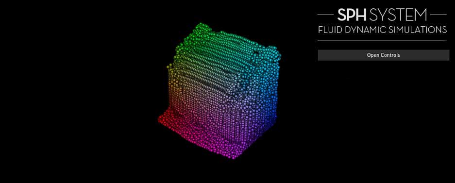
Finally here are some images of our first breaking dam simulation.

Simulation showing the densities of each particle.

Simulation showing the position field of the particles.

Simulation showing the velocity field of the particles.
We would like to thanks AlteredQ for the help of testing the simulator, sadly we couldn´t find a solution for some configurations, so we have made a video if you can not play the simulation correctly. The simulations works fine with these configurations:
– Mac OS (Lion) with AMD Radeom HD 6970M 2Gb using Google Chrome and Firefox.
– Mac OS (Snow Leopard) with AMD Radeom HD 6750M 1Gb using Google Chrome and Firefox.
– Mac Os (Leopard) with Nvidia 8800 GT 512Mb using Firefox.
– Max Os (Snow Leopard) with Nvidia 9600GT 512Mb using Google Chrome and Firefox.
– Windows XP with Nvidia 8800GT 512Mb using Google Chrome.
– Windows 7 with AMD Radeom HD 6750M 1Gb using Google Chrome and Firefox.
– Windows 7 with Nvidia 9600GT 512Mb using Google Chrome and Firefox.
Feel free to try it, and if it´s broken please let us know your configuration, and what exactly you have seen while you played the simulation. It is our first version of the implementation, so we hope to make it faster using a more convenient neighborhood search. We hope that future posts will go on two branches, SPH optimizations and particles rendering using marching cubes.